Feature Selection 기법 알아보기

시작하며

ML 모델링을 하는 데 있어 어떤 특징(Feature)을 중점적으로 학습하는지는 성능에 지대한 영향을 미친다. 이를 위해 EDA(Exploratory Data Analysis)라는 과정을 통해 선제적으로 데이터를 분석하고 시각화하여 전반적인 데이터 전처리 전략을 결정하기도 한다.

하지만 이 Feature가 수만 개 혹은 그 이상이 된다면 어떻게 해야 할까? 그 많은 특성들을 모두 하나하나 EDA를 통해 분석하기란 쉽지 않다. 시각화를 통한 선별은 꼼꼼하게 데이터를 살펴볼 수 있지만 그만큼의 시간과 노동력을 필요로 하기 때문이다.

이번 포스팅에서는 PoC 프로젝트에서 이러한 문제를 해결하기 위해 Feature Selection 과정을 자동화하여 통계적으로 어떻게 대상 Feature 군집을 축소하였는지를 기록으로 남기고자 한다.

Feature Selection

Feature Selection vs Feature Extraction

본격적으로 들어가기에 앞서, Feature Selection이란 무엇인지에 대해 먼저 정리해 보고자 한다. Feature Selection의 정의는 다음과 같다.

feature selection is the process of selecting a subset of relevant features (variables, predictors) for use in model construction “Feature selection은 모델 구축에 사용하기 위해 관련 있는 특징(변수, 예측 변수)의 일부를 선택하는 과정이다.”

• 유사한 개념으로는 Feature Extraction이 있다.

Feature extraction is a machine learning technique that reduces the number of resources required for processing while retaining significant or relevant information. “Feature extraction은 처리에 필요한 자원을 줄이면서 중요한 또는 관련된 정보를 유지하는 머신 러닝 기법이다.”

비슷한 의미로 보이지만, Feature Selection은 Original Set을 그대로 사용하는 데 반해, Feature Extraction은 Original Set을 새로운 Feature로 변환시켜 사용한다는 차이가 있다.

Feature Selection Methods

Feature Selection의 방법은 보통 3가지 분류로 나뉜다. Filter methods, Wrapper methods, 그리고 Embedded methods인데 하나하나 살펴보도록 하겠다.

방법 1. Filter Method (관련성을 찾는 방법)

• 특징
  • Filter Method는 통계적 측정 방법을 사용하여 피처들의 상관관계를 알아낸다.
  • 계산속도가 빠르고 피처 간 상관관계를 알아내는 데 적합하기 때문에 Wrapper method를 사용하기 전에 전처리하는 데 사용된다.
  • 중복되고 상관 관계가 있는 피처를 제거하는 데 유용하다.
• 종류
  • Chi-Square Test: 일반적으로 범주형 변수 간의 관계를 검정하는 데 사용된다.
  • Correlation: 대표적인 피어슨 상관계수는 두 연속 변수 간의 연관성과 관계의 방향을 정량화하는 척도다.
  • Variance Threshold: 데이터의 분산(Variance)이 설정한 임계값(threshold)보다 낮은 특성을 제거하는 방법이다.
  • Mutual Information: 특성과 타겟 변수 간의 상호의존성을 고려한 비선형 관계 측정에 사용된다.

Tip

Correlation 계수 정리

• 수치형-수치형
  • Pearson: 두 연속형 변수 간의 선형 상관 관계를 측정 (값의 범위: -1 ~ 1). 정규분포를 가정.
  • Spearman: 순위를 기반으로 비선형 관계도 측정 가능. 이상치에 덜 민감.
  • Kendall: 순위 일치 정도를 측정하며, 데이터가 작거나 이상치가 많을 때 적합.
• 수치형-범주형 / 범주형-수치형
  • Point-Biserial: 이분형(2개의 범주) 변수와 연속형 변수 간의 상관 관계를 측정.
  • ANOVA: 범주형 독립 변수와 연속형 종속 변수 간의 평균 차이를 분석하여 관계를 확인.
• 범주형-범주형
  • Cramér’s V: 두 범주형 변수 간의 관계를 측정 (카이제곱 통계 기반).
  • Phi 계수: 2x2 범주형 데이터 테이블에 사용.

방법 2. Wrapper Method: 유용성을 측정한 방법

• 특징
  • Wrapper Method는 탐욕 알고리즘이라고도 하며 반복적인 방식으로 하위 집합의 피처를 사용하여 알고리즘을 학습한다.
  • 예측 모델을 사용하여 피처 subset을 계속 테스트하는 방식이다.
• 종류
  • Forward selection: 처음에 빈 피처 세트로 시작하여 각 반복 후에 모델을 가장 잘 개선하는 피처를 계속 추가한다. 추가해도 모델의 성능이 개선되지 않을 때 중지한다.
  • Backward elimination: Forward와 반대로 처음에 모든 피처로 시작하고 각 반복 후에 가장 중요하지 않은 피처를 제거한다. 중지 기준은 동일하다.
  • Bi-directional elimination: 전방 선택과 후방 제거 기술을 동시에 사용하는 방법이다.
  • Exhaustive selection: 모든 가능한 하위 집합을 생성하고, 각 하위 집합에 대한 학습 알고리즘을 빌드하며 모델의 성능이 가장 좋은 하위 집합을 선택한다.
  • Recursive elimination: 점점 더 작은 피처 세트를 재귀적으로 고려하여 피처를 선택한다. 추정자는 초기 피처 세트에서 학습되고 feature_importance_attribute를 사용하여 중요도를 얻는다. 그 후 가장 중요하지 않은 피처는 현재 피처 세트에서 제거되어 필요한 수의 피처가 남는다.

방법 3. Embedded Method: 유용성을 측정하지만 내장 metric을 사용하는 방법

• 특징
  • Embedded Method는 학습 알고리즘의 일부로 혼합되어 자체 내장 피처를 선택하는 방식이다.
  • 모델의 정확도에 기여하는 피처를 학습한다.
• 종류
  • Tree-based methods: 랜덤 포레스트, 그래디언트 부스팅과 같은 방법은 피처 중요도를 제공하여 피처를 선택한다. 피처 중요도는 대상 피처에 영향을 미치는 데 어떤 피처가 더 중요한지 알려준다.
  • Regularization: 모델의 과적합을 방지하기 위해 머신 러닝 모델의 다양한 매개변수에 페널티를 추가한다. Lasso(L1 정규화)와 Elastic net(L1 및 L2 정규화)을 사용한다.

또다른 고려점 - Feature Type

위 여러 가지 Feature Selection Methods 중에서 간단하고 빠르게, 반복적으로 다수의 Feature들을 분석하여 면밀하게 분석해 볼 Feature들을 걸러내는 것이 목적이었다. 따라서 모든 Subset 집합을 확인하는 방식(wrapper)은 제외하고, 필터링(filter)과 트리 내장 함수(embedded) 방식을 사용하기로 하였다.

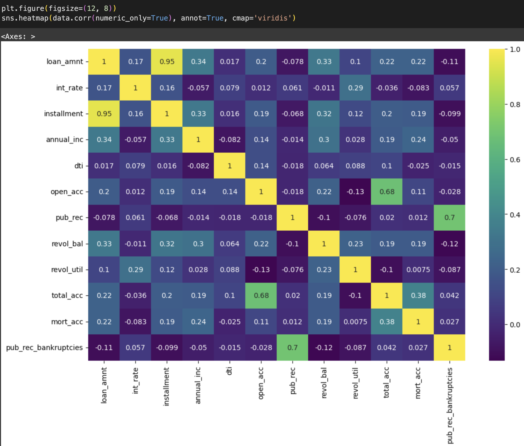
제일 처음 시도한 것은 상관계수 분석이다. 타겟 값을 기준으로 히트맵을 그려보면 위와 같이 나타나는 것을 볼 수 있다. 이를 통해 일차적으로 상관성이 나타나지 않는 칼럼들이나, loan_amnt <-> installment 같이 다중공선성 문제가 발생할 여지가 있는 컬럼들은 미리 소거할 수 있다.

하지만 상관계수 방법만으로는 한계가 있으므로 Feature Selection에서는 데이터의 특징에 따라 더 다양한 알고리즘들이 소개되어 있다. 이는 상황에 맞게 선택하면 되는데, 대표적으로는 피처와 타겟 변수 간의 선형/비선형 여부에 따라 아래와 같은 방법을 사용할 수 있다.

선형 관계 탐색

1. Numeric-Numeric (숫자형 vs 숫자형)

• 검정 방식: Pearson Correlation, Spearman Correlation
• 설명:
  • Pearson Correlation: 두 숫자형 변수의 선형 관계를 측정.
  • Spearman Correlation: 두 숫자형 변수의 순위 간 관계를 측정하며, 비선형적인 단조(monotonic) 관계도 일부 반영.

from scipy.stats import pearsonr, spearmanr
 
pearson_corr, _ = pearsonr(feature, target)
spearman_corr, _ = spearmanr(feature, target)

2. Numeric-Categorical (숫자형 vs 범주형)

• 검정 방식: ANOVA F-test, Point-Biserial Correlation
• 설명:
  • ANOVA F-test: 범주형 타겟 변수(이진 또는 다중 클래스)와 숫자형 feature 간의 선형 관계를 검정.
  • Point-Biserial Correlation: 이진 타겟 변수와 숫자형 feature 간의 선형 관계를 측정.

from sklearn.feature_selection import mutual_info_classif
 
mi_scores = mutual_info_classif(X, y)

비선형 관계 탐색

1. Numeric-Numeric (숫자형 vs 숫자형)

• 검정 방식: Mutual Information, Distance Correlation
• 설명:
  • Mutual Information: 두 변수 간의 상호 정보량을 계산하여 비선형 관계를 측정.
  • Distance Correlation: 두 숫자형 변수 간의 독립 여부를 비선형 관계까지 포함해 평가.

from sklearn.feature_selection import mutual_info_regression
 
mi_scores = mutual_info_regression(X, y)

2. Numeric-Categorical (숫자형 vs 범주형)

• 검정 방식: Mutual Information, Decision Tree Feature Importance
• 설명:
  • Mutual Information: 숫자형 feature와 범주형 타겟 간의 비선형 관계를 측정.
  • Decision Tree Feature Importance: Tree-based 모델(XGBoost, Random Forest 등)에서 feature 중요도를 계산.

from sklearn.feature_selection import mutual_info_classif
 
mi_scores = mutual_info_classif(X, y)

3. Categorical-Categorical (범주형 vs 범주형)

• 검정 방식: Chi-Square Test, Mutual Information
• 설명:
  • Chi-Square Test: 두 범주형 변수 간의 독립 여부를 검정.
  • Mutual Information: 범주형 feature와 타겟 간의 비선형 관계를 측정.

from sklearn.feature_selection import chi2
 
chi2_scores, p_values = chi2(X, y)

Feature Selection Methods 정리

이번에 풀려고 한 문제는 비식별화 데이터를 통한 타행 대출 적정성 여부 판단이었고, 따로 대출한도는 계산할 필요 없이 True/False만 가려주면 되는 문제였다. 따라서 타겟 변수는 이진(Categorical) 데이터로 고정되었고 대조하고자 하는 Feature는 수치형, 범주형 모두 가능한 상황이었다. 따라서 1) 범주형 - 수치형에 대한 탐색, 2) 범주형 - 범주형에 대한 탐색의 두 가지 케이스로 나누어 진행했다.

1. 범주형 - 수치형

• Mutual Information (MI)

  • 타겟(범주형)과 피처(수치형) 간의 비선형 관계까지 평가 가능.
  • Scikit-learn의 mutual_info_classif 함수로 구현.

• Tree-based Feature Importance (Random Forest, XGBoost)

  • 고차원 데이터에서 비선형 관계를 고려하기 때문에 널리 사용.
  • 특히 엔지니어링이 어려운 데이터에서 강력한 성능.

2. 범주형 - 범주형

• 선택 방법: Chi-squared Test (카이제곱 검정)
  • 범주형 타겟과 범주형 피처 간의 독립성을 평가.
  • 피처와 타겟 간의 기대값과 관측값 차이를 기반으로 관계를 분석.

Feature Selection Methods 맛보기

이제 이론을 토대로 Feature Selection을 적용해 보겠다. PoC에서는 수만 개의 Feature 군집에서 유효한 Feature들을 1차적으로 걸러내는 데 사용하였지만 외부로 내용을 가져올 수는 없으므로 Kaggle에서 테스트했던 내용을 가지고 왔다.

위 Prediction 과정에서 사용하는 DataSet은 아래 27개의 Feature와 1개의 Target Feature를 가지고 있다.

number	LoanStatNew	Description
0	loan_amnt	The listed amount of the loan applied for by the borrower. If at some point in time, the credit department reduces the loan amount, then it will be reflected in this value.
1	term	The number of payments on the loan. Values are in months and can be either 36 or 60.
2	int_rate	Interest Rate on the loan
3	installment	The monthly payment owed by the borrower if the loan originates.
4	grade	LC assigned loan grade
5	sub_grade	LC assigned loan subgrade
6	emp_title	The job title supplied by the Borrower when applying for the loan.*
7	emp_length	Employment length in years. Possible values are between 0 and 10 where 0 means less than one year and 10 means ten or more years.
8	home_ownership	The home ownership status provided by the borrower during registration or obtained from the credit report. Our values are: RENT, OWN, MORTGAGE, OTHER
9	annual_inc	The self-reported annual income provided by the borrower during registration.
10	verification_status	Indicates if income was verified by LC, not verified, or if the income source was verified
11	issue_d	The month which the loan was funded
12	loan_status	Current status of the loan
13	purpose	A category provided by the borrower for the loan request.
14	title	The loan title provided by the borrower
15	zip_code	The first 3 numbers of the zip code provided by the borrower in the loan application.
16	addr_state	The state provided by the borrower in the loan application
17	dti	A ratio calculated using the borrower’s total monthly debt payments on the total debt obligations, excluding mortgage and the requested LC loan, divided by the borrower’s self-reported monthly income.
18	earliest_cr_line	The month the borrower’s earliest reported credit line was opened
19	open_acc	The number of open credit lines in the borrower’s credit file.
20	pub_rec	Number of derogatory public records
21	revol_bal	Total credit revolving balance
22	revol_util	Revolving line utilization rate, or the amount of credit the borrower is using relative to all available revolving credit.
23	total_acc	The total number of credit lines currently in the borrower’s credit file
24	initial_list_status	The initial listing status of the loan. Possible values are – W, F
25	application_type	Indicates whether the loan is an individual application or a joint application with two co-borrowers
26	mort_acc	Number of mortgage accounts.
27	pub_rec_bankruptcies	Number of public record bankruptcies

1. MI 데이터 확인

# Mutual Information (MI)
from sklearn.feature_selection import mutual_info_classif
 
# MI 적용
X = data[numeric_columns]
y = data['loan_status']
 
valid_indices = X.dropna().index.intersection(y.dropna().index)
 
X_cleaned = X.loc[valid_indices]
y_cleaned = y.loc[valid_indices]
 
mi_scores = mutual_info_classif(X_cleaned, y_cleaned, discrete_features=True)
mi_scores = pd.Series(mi_scores, index=X.columns)
print(mi_scores)

2. Feature Importance 데이터 확인

# XGBoost 분류 모델 학습
xgb_clf = XGBClassifier(use_label_encoder=False, eval_metric='logloss', random_state=42)
xgb_clf.fit(X, y)
 
# Feature Importance 추출
feature_importances = pd.Series(xgb_clf.feature_importances_, index=X.columns)
print("XGBoost Feature Importances:")
print(feature_importances)
 
import matplotlib.pyplot as plt
 
# Feature Importance 시각화
feature_importances.sort_values(ascending=False).plot.bar()
plt.title('Feature Importances')
plt.ylabel('Importance Score')
plt.show()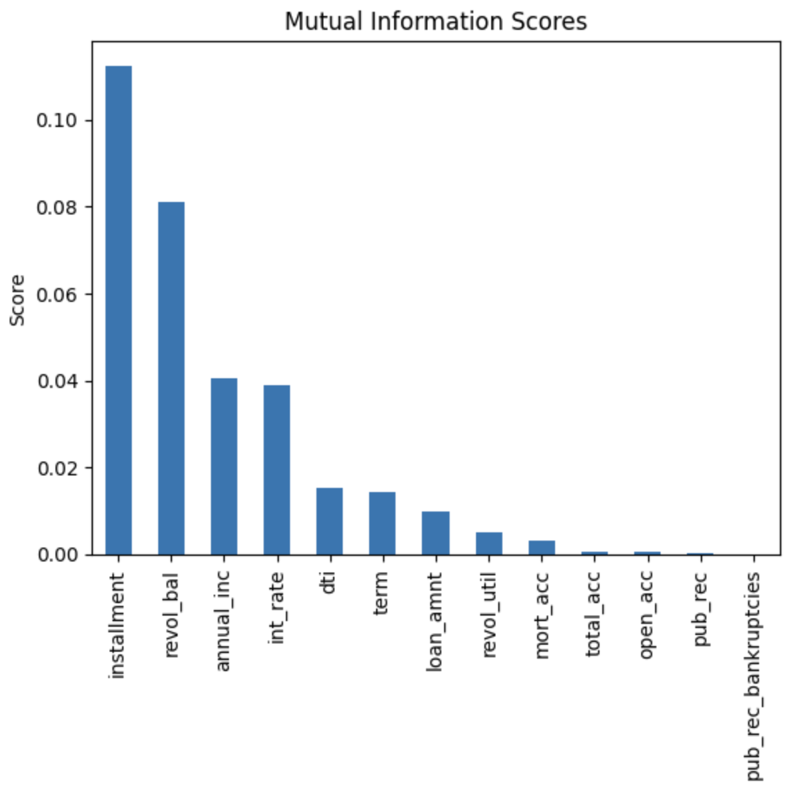

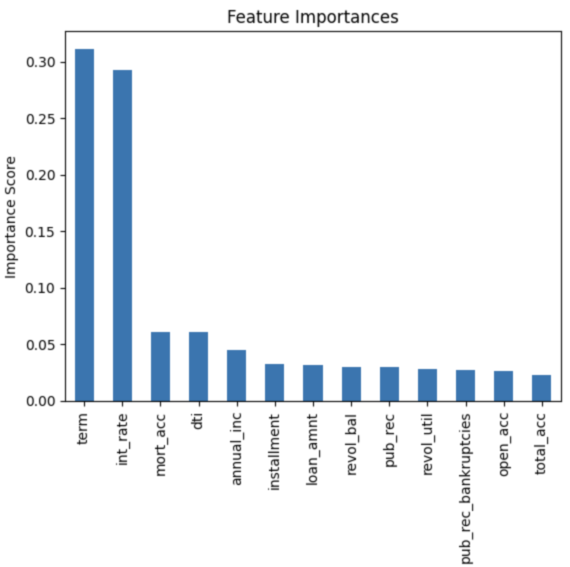
위 그래프는 MI, Feature Selection을 각각 수행한 후 이를 시각화하여 나타낸 그래프다. MI에서는 installment ~ int_rate 값이 높게 나타났고 Feature Importance에서는 term, int_rate이 높게 나타났다.

3. Chi-squared 데이터 확인

# chi^2
import pandas as pd
from scipy.stats import chi2_contingency
 
features = columns
results = {}
 
for feature in features:
    contingency_table = pd.crosstab(data[feature], data['loan_status'])
    chi2, p, _, _ = chi2_contingency(contingency_table)
    results[feature] = {'Chi-Square Statistic': chi2, 'p-value': p}
 
# 결과를 데이터프레임으로 보기 좋게 정리
chi2_results = pd.DataFrame(results).T
print(chi2_results)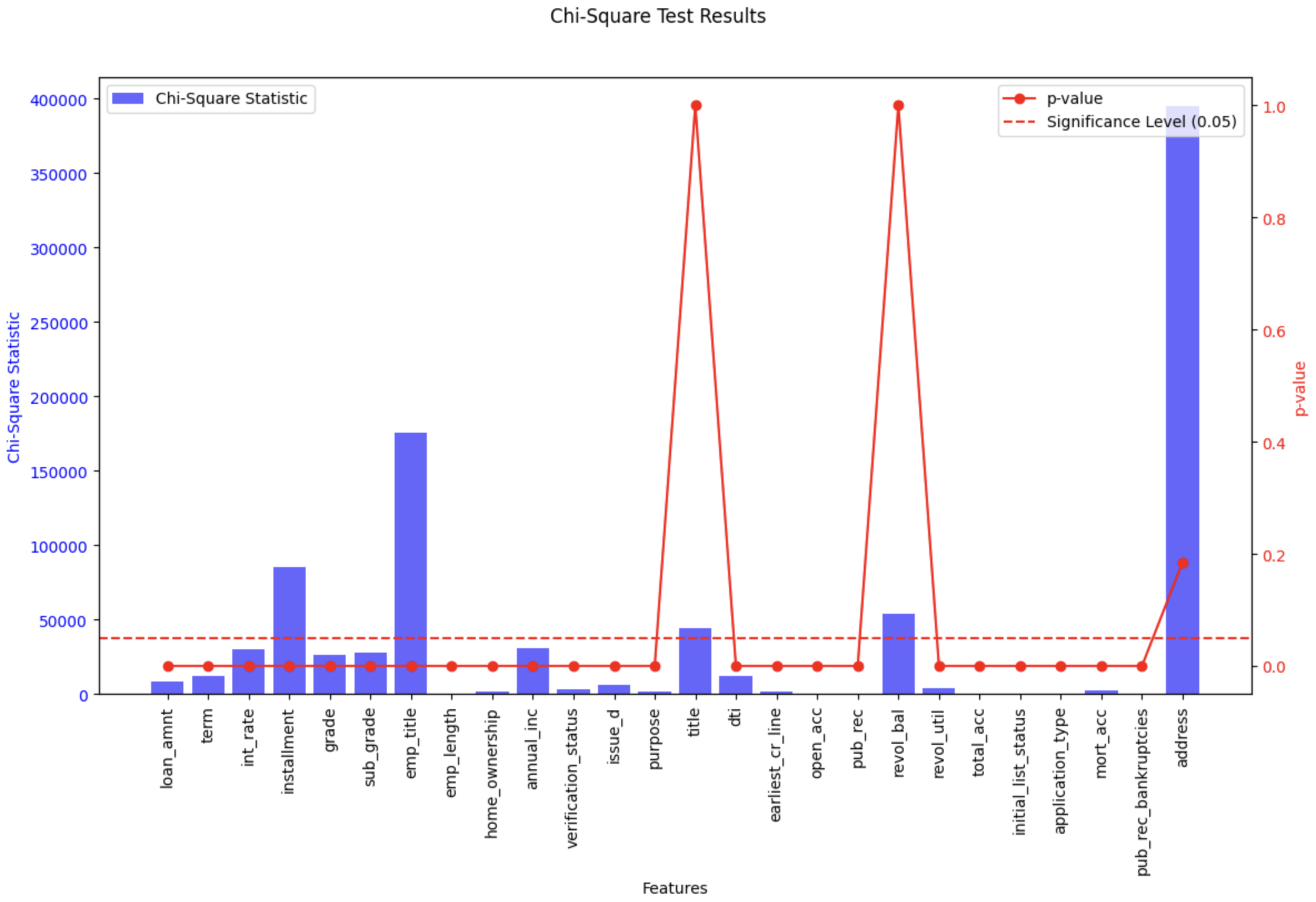

위 그래프는 카이제곱 분포에 대한 각 칼럼별 수치값을 나타낸 것이다. Chi-Square 통계량과 p-value 값을 보고 서로 연관성이 있는지, 그리고 통계적으로 유의미한지(p-value ≤ 0.05)를 보여준다. installment와 emp_title은 여기서도 유의미한 값을 나타내고 있다. 반면 p-value만 지나치게 높은 title, revol_bal은 통계적으로 유의미하지 않으며, address 역시 통계량은 높지만 p-value 값이 높아 통계적으로 유의미하지 않다.

정리하며

이번에는 Feature Selection 기법들을 알아보고, 구체적인 분석 기법을 정리한 후 binary-classification에 적당한 기법들을 추려 적용해 보았다. 각 Feature들이 통계적으로 유의미한 값인지를 EDA 이전 과정에서 선제적으로 확인하고자 할 때 Feature Selection 기법은 좋은 선택지가 될 것으로 보인다. 테스트 환경에서는 물론 실제 데이터를 통해 모델링을 할 때에도 짧은 시간에 유의미한 결과를 만들어 낼 수 있었다. 이번 포스팅에는 함께 정리하지는 못했지만 scikit-learn 기반의 Feature Selection 외에도 sparkML을 통한 Feature Selection도 거의 동일한 개념 하에 가능하다. 관심 있는 분들은 이곳을 참조하면 된다.

추가로 통계 관련 분석 코드들은 주로 라이브러리를 많이 사용한다. 편하게 가져다 쓰기만 하면 되는데 그러다 보니 구체적인 동작 원리는 지나치기 쉬운 것 같다. 시간이 된다면 다음번에는 기초통계학과 관련된 내용을 한번 정리해봐야겠다.

참고문헌

• geeksforgeeks feature selection 개요
• scikit-learn feature selection 공식페이지
• Feature Selection 방법론 잘 정리된 글
• Feature Extraction vs Feature Selection
• https://www.kaggle.com/code/faressayah/lending-club-loan-defaulters-prediction
• https://scikit-learn.org/1.5/modules/feature_selection.html
• https://spark.apache.org/docs/latest/ml-features.html#feature-selectors